69. A Lake Model of Employment and Unemployment#
In addition to what’s in Anaconda, this lecture will need the following libraries:
!pip install quantecon jax
69.1. Overview#
This lecture describes what has come to be called a lake model.
The lake model is a basic tool for modeling unemployment.
It allows us to analyze
flows between unemployment and employment
how these flows influence steady state employment and unemployment rates
It is a good model for interpreting monthly labor department reports on gross and net jobs created and destroyed.
The “lakes” in the model are the pools of employed and unemployed.
The “flows” between the lakes are caused by
firing and hiring
entry and exit from the labor force
For the first part of this lecture, the parameters governing transitions into and out of unemployment and employment are exogenous.
Later, we’ll determine some of these transition rates endogenously using the McCall search model.
We’ll also use some nifty concepts like ergodicity, which provides a fundamental link between cross-sectional and long run time series distributions.
These concepts will help us build an equilibrium model of ex-ante homogeneous workers whose different luck generates variations in their ex post experiences.
Let’s start with some imports:
import matplotlib.pyplot as plt
import jax
import jax.numpy as jnp
from typing import NamedTuple
from quantecon.distributions import BetaBinomial
from functools import partial
import jax.scipy.stats as stats
Matplotlib is building the font cache; this may take a moment.
69.1.1. Prerequisites#
Before working through what follows, we recommend you read the lecture on finite Markov chains.
You will also need some basic linear algebra and probability.
69.2. The model#
The economy is inhabited by a very large number of ex-ante identical workers.
The workers live forever, spending their lives moving between unemployment and employment.
Their rates of transition between employment and unemployment are governed by the following parameters:
\(\lambda\), the job finding rate for currently unemployed workers
\(\alpha\), the dismissal rate for currently employed workers
\(b\), the entry rate into the labor force
\(d\), the exit rate from the labor force
The growth rate of the labor force evidently equals \(g=b-d\).
69.2.1. Aggregate variables#
We want to derive the dynamics of the following aggregates:
\(E_t\), the total number of employed workers at date \(t\)
\(U_t\), the total number of unemployed workers at \(t\)
\(N_t\), the number of workers in the labor force at \(t\)
We also want to know the values of the following objects:
The employment rate \(e_t := E_t/N_t\).
The unemployment rate \(u_t := U_t/N_t\).
(Here and below, capital letters represent aggregates and lowercase letters represent rates)
69.2.2. Laws of motion for stock variables#
We begin by constructing laws of motion for the aggregate variables \(E_t,U_t, N_t\).
Of the mass of workers \(E_t\) who are employed at date \(t\),
\((1-d)E_t\) will remain in the labor force
of these, \((1-\alpha)(1-d)E_t\) will remain employed
Of the mass of workers \(U_t\) workers who are currently unemployed,
\((1-d)U_t\) will remain in the labor force
of these, \((1-d) \lambda U_t\) will become employed
Therefore, the number of workers who will be employed at date \(t+1\) will be
A similar analysis implies
The value \(b(E_t+U_t)\) is the mass of new workers entering the labor force unemployed.
The total stock of workers \(N_t=E_t+U_t\) evolves as
Letting \(X_t := \left(\begin{matrix}U_t\\E_t\end{matrix}\right)\), the law of motion for \(X\) is
This law tells us how total employment and unemployment evolve over time.
69.2.3. Laws of motion for rates#
Now let’s derive the law of motion for rates.
To get these we can divide both sides of \(X_{t+1} = A X_t\) by \(N_{t+1}\) to get
Letting
we can also write this as
You can check that \(e_t + u_t = 1\) implies that \(e_{t+1}+u_{t+1} = 1\).
This follows from the fact that the columns of \(\hat A\) sum to 1.
69.3. Implementation#
Let’s code up these equations.
To do this we’re going to use a class that we’ll call LakeModel that stores the primitives \(\alpha, \lambda, b, d\)
class LakeModel(NamedTuple):
    """
    Parameters for the lake model
    """
    λ: float = 0.283
    α: float = 0.013
    b: float = 0.0124
    d: float = 0.00822
We will also use a specialized function to generate time series in an efficient JAX-compatible manner.
(Iteratively generating time series is somewhat nontrivial in JAX because arrays are immutable.)
@partial(jax.jit, static_argnames=['f', 'num_steps'])
def generate_path(f, initial_state, num_steps, **kwargs):
    """
    Generate a time series by repeatedly applying an update rule.

    Given a map f, initial state x_0, and a set of model parameter θ, this
    function computes and returns the sequence {x_t}_{t=0}^{T-1} when

        x_{t+1} = f(x_t, t, θ)

    Args:
        f: Update function mapping (x_t, t, θ) -> x_{t+1}
        initial_state: Initial state x_0
        num_steps: Number of time steps T to simulate
        **kwargs: Optional extra arguments passed to f

    Returns:
        Array of shape (dim(x), T) containing the time series path
        [x_0, x_1, x_2, ..., x_{T-1}]
    """

    def update_wrapper(state, t):
        """
        Wrapper function that adapts f for use with JAX scan.
        """
        next_state = f(state, t, **kwargs)
        return next_state, state

    _, path = jax.lax.scan(update_wrapper,
                    initial_state, jnp.arange(num_steps))
    return path.T
Now we can compute the matrices and simulate the dynamics.
@jax.jit
def compute_matrices(model: LakeModel):
    """Compute the transition matrices A and A_hat for the model."""
    λ, α, b, d = model.λ, model.α, model.b, model.d
    g = b - d
    A = jnp.array([[(1-d) * (1-λ) + b,      (1 - d) * α + b],
                   [        (1-d) * λ,      (1 - d) * (1 - α)]])
    A_hat = A / (1 + g)
    return A, A_hat, g


@jax.jit
def stock_update(current_stocks, time_step, model):
    """
    Apply transition matrix to get next period's stocks.
    """
    A, A_hat, g = compute_matrices(model)
    next_stocks = A @ current_stocks
    return next_stocks

@jax.jit
def rate_update(current_rates, time_step, model):
    """
    Apply normalized transition matrix for next period's rates.
    """
    A, A_hat, g = compute_matrices(model)
    next_rates = A_hat @ current_rates
    return next_rates
We create two instances, one with \(α=0.013\) and another with \(α=0.03\)
model = LakeModel()
model_new = LakeModel(α=0.03)

print(f"Default α: {model.α}")
A, A_hat, g = compute_matrices(model)
print(f"A matrix:\n{A}")
Default α: 0.013
A matrix:
[[0.7235062  0.02529314]
 [0.28067374 0.97888684]]
A_new, A_hat_new, g_new = compute_matrices(model_new)
print(f"New α: {model_new.α}")
print(f"New A matrix:\n{A_new}")
New α: 0.03
New A matrix:
[[0.7235062  0.0421534 ]
 [0.28067374 0.9620266 ]]
69.3.1. Aggregate dynamics#
Let’s run a simulation under the default parameters (see above) starting from \(X_0 = (12, 138)\).
N_0 = 150      # Population
e_0 = 0.92     # Initial employment rate
u_0 = 1 - e_0  # Initial unemployment rate
T = 50         # Simulation length

U_0 = u_0 * N_0
E_0 = e_0 * N_0

fig, axes = plt.subplots(3, 1, figsize=(10, 8))
X_0 = jnp.array([U_0, E_0])
X_path = generate_path(stock_update, X_0, T, model=model)

axes[0].plot(X_path[0, :], lw=2)
axes[0].set_title('unemployment')

axes[1].plot(X_path[1, :], lw=2)
axes[1].set_title('employment')

axes[2].plot(X_path.sum(0), lw=2)
axes[2].set_title('labor force')

plt.tight_layout()
plt.show()
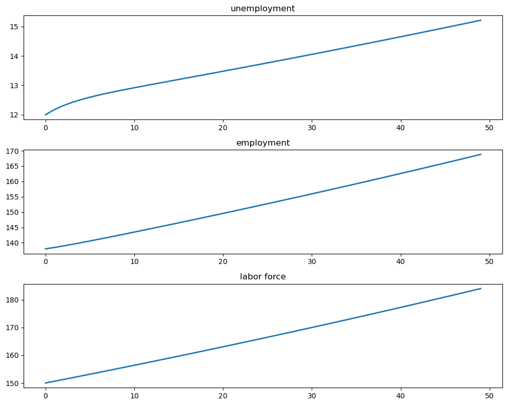
The aggregates \(E_t\) and \(U_t\) don’t converge because their sum \(E_t + U_t\) grows at rate \(g\).
On the other hand, the vector of employment and unemployment rates \(x_t\) can be in a steady state \(\bar x\) if there exists an \(\bar x\) such that
\(\bar x = \hat A \bar x\)
the components satisfy \(\bar e + \bar u = 1\)
This equation tells us that a steady state level \(\bar x\) is an eigenvector of \(\hat A\) associated with a unit eigenvalue.
The following function can be used to compute the steady state.
@jax.jit
def rate_steady_state(model: LakeModel):
    r"""
    Finds the steady state of the system :math:`x_{t+1} = \hat A x_{t}`
    by computing the eigenvector corresponding to the unit eigenvalue.
    """
    A, A_hat, g = compute_matrices(model)
    eigenvals, eigenvec = jnp.linalg.eig(A_hat)

    # Find the eigenvector corresponding to eigenvalue 1
    unit_idx = jnp.argmin(jnp.abs(eigenvals - 1.0))

    # Get the corresponding eigenvector
    steady_state = jnp.real(eigenvec[:, unit_idx])

    # Normalize to ensure positive values and sum to 1
    steady_state = jnp.abs(steady_state)
    steady_state = steady_state / jnp.sum(steady_state)

    return steady_state
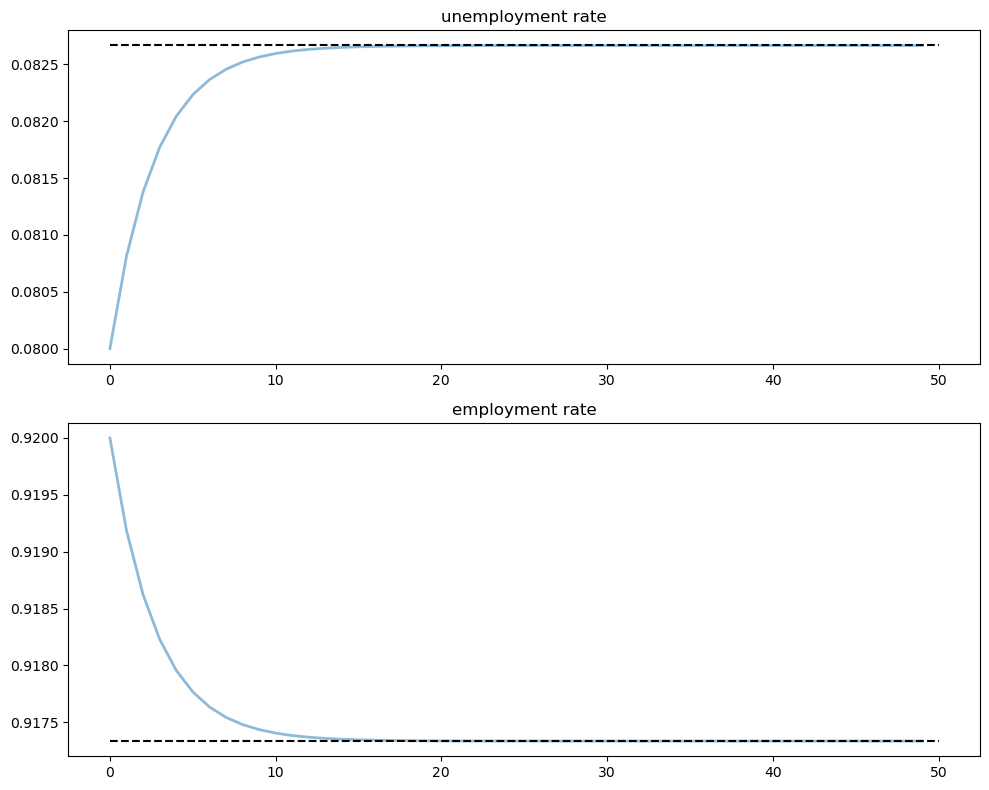
We also have \(x_t \to \bar x\) as \(t \to \infty\) provided that the remaining eigenvalue of \(\hat A\) has modulus less than 1.
This is the case for our default parameters:
A, A_hat, g = compute_matrices(model)
e, f = jnp.linalg.eigvals(A_hat)
print(f"Eigenvalue magnitudes: {abs(e):.2f}, {abs(f):.2f}")
Eigenvalue magnitudes: 0.70, 1.00
Let’s look at the convergence of the unemployment and employment rates to steady state levels (dashed black line)
xbar = rate_steady_state(model)

fig, axes = plt.subplots(2, 1, figsize=(10, 8))
x_0 = jnp.array([u_0, e_0])
x_path = generate_path(rate_update, x_0, T, model=model)

titles = ['unemployment rate', 'employment rate']

for i, title in enumerate(titles):
    axes[i].plot(x_path[i, :], lw=2, alpha=0.5)
    axes[i].hlines(xbar[i], 0, T, 'black', '--')
    axes[i].set_title(title)

plt.tight_layout()
plt.show()
69.4. Dynamics of an individual worker#
An individual worker’s employment dynamics are governed by a finite state Markov process.
The worker can be in one of two states:
\(s_t=0\) means unemployed
\(s_t=1\) means employed
Let’s start off under the assumption that \(b = d = 0\).
The associated transition matrix is then
Let \(\psi_t\) denote the marginal distribution over employment/unemployment states for the worker at time \(t\).
As usual, we regard it as a row vector.
We know from an earlier discussion that \(\psi_t\) follows the law of motion
We also know from the lecture on finite Markov chains that if \(\alpha \in (0, 1)\) and \(\lambda \in (0, 1)\), then \(P\) has a unique stationary distribution, denoted here by \(\psi^*\).
The unique stationary distribution satisfies
Not surprisingly, probability mass on the unemployment state increases with the dismissal rate and falls with the job finding rate.
69.4.1. Ergodicity#
Let’s look at a typical lifetime of employment-unemployment spells.
We want to compute the average amounts of time an infinitely lived worker would spend employed and unemployed.
Let
and
(As usual, \(\mathbb 1\{Q\} = 1\) if statement \(Q\) is true and 0 otherwise)
These are the fraction of time a worker spends unemployed and employed, respectively, up until period \(T\).
If \(\alpha \in (0, 1)\) and \(\lambda \in (0, 1)\), then \(P\) is ergodic, and hence we have
with probability one.
Inspection tells us that \(P\) is exactly the transpose of \(\hat A\) under the assumption \(b=d=0\).
Thus, the percentages of time that an infinitely lived worker spends employed and unemployed equal the fractions of workers employed and unemployed in the steady state distribution.
69.4.2. Convergence rate#
How long does it take for time series sample averages to converge to cross-sectional averages?
We can investigate this by simulating the Markov chain.
Let’s plot the path of the sample averages over 5,000 periods
@jax.jit
def markov_update(state, t, P, keys):
    """
    Sample next state from transition probabilities.
    """
    probs = P[state]
    state_new = jax.random.choice(keys[t],
                        a=jnp.arange(len(probs)),
                        p=probs)
    return state_new

model_markov = LakeModel(d=0, b=0)
T = 5000  # Simulation length

α, λ = model_markov.α, model_markov.λ

P = jnp.array([[1 - λ,        λ],
              [    α,    1 - α]])

xbar = rate_steady_state(model_markov)

# Simulate the Markov chain
key = jax.random.PRNGKey(0)
keys = jax.random.split(key, T)
s_path = generate_path(markov_update, 1, T, P=P, keys=keys)

fig, axes = plt.subplots(2, 1, figsize=(10, 8))
s_bar_e = jnp.cumsum(s_path) / jnp.arange(1, T+1)
s_bar_u = 1 - s_bar_e

to_plot = [s_bar_u, s_bar_e]
titles = ['percent of time unemployed', 'percent of time employed']

for i, plot in enumerate(to_plot):
    axes[i].plot(plot, lw=2, alpha=0.5)
    axes[i].hlines(xbar[i], 0, T, 'r', '--')
    axes[i].set_title(titles[i])

plt.tight_layout()
plt.show()
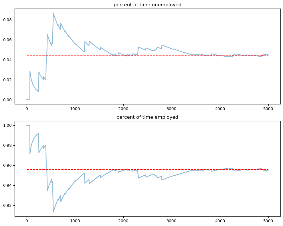
The stationary probabilities are given by the dashed red line.
In this case it takes much of the sample for these two objects to converge.
This is largely due to the high persistence in the Markov chain.
69.5. Endogenous job finding rate#
We now make the hiring rate endogenous.
The transition rate from unemployment to employment will be determined by the McCall search model [McCall, 1970].
All details relevant to the following discussion can be found in our treatment of that model.
69.5.1. Reservation wage#
The most important thing to remember about the model is that optimal decisions are characterized by a reservation wage \(\bar w\)
If the wage offer \(w\) in hand is greater than or equal to \(\bar w\), then the worker accepts.
Otherwise, the worker rejects.
As we saw in our discussion of the model, the reservation wage depends on the wage offer distribution and the parameters
\(\alpha\), the separation rate
\(\beta\), the discount factor
\(\gamma\), the offer arrival rate
\(c\), unemployment compensation
69.5.2. Linking the McCall search model to the lake model#
Suppose that all workers inside a lake model behave according to the McCall search model.
The exogenous probability of leaving employment remains \(\alpha\).
But their optimal decision rules determine the probability \(\lambda\) of leaving unemployment.
This is now
69.5.3. Fiscal policy#
We can use the McCall search version of the Lake Model to find an optimal level of unemployment insurance.
We assume that the government sets unemployment compensation \(c\).
The government imposes a lump-sum tax \(\tau\) sufficient to finance total unemployment payments.
To attain a balanced budget at a steady state, taxes, the steady state unemployment rate \(u\), and the unemployment compensation rate must satisfy
The lump-sum tax applies to everyone, including unemployed workers.
Thus, the post-tax income of an employed worker with wage \(w\) is \(w - \tau\).
The post-tax income of an unemployed worker is \(c - \tau\).
For each specification \((c, \tau)\) of government policy, we can solve for the worker’s optimal reservation wage.
This determines \(\lambda\) via (69.1) evaluated at post tax wages, which in turn determines a steady state unemployment rate \(u(c, \tau)\).
For a given level of unemployment benefit \(c\), we can solve for a tax that balances the budget in the steady state
To evaluate alternative government tax-unemployment compensation pairs, we require a welfare criterion.
We use a steady state welfare criterion
where the notation \(V\) and \(U\) is as defined in the McCall search model lecture.
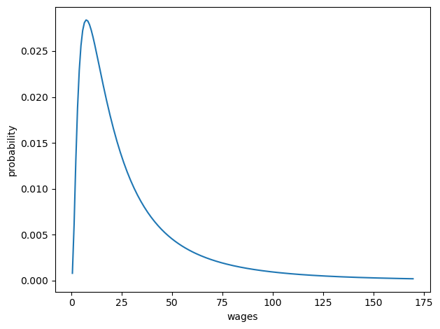
The wage offer distribution will be a discretized version of the lognormal distribution \(LN(\log(20),1)\), as shown in the next figure
def create_wage_distribution(max_wage: float,
                             wage_grid_size: int,
                             log_wage_mean: float):
    """Create wage distribution"""
    w_vec_temp = jnp.linspace(1e-8, max_wage,
                                wage_grid_size + 1)
    cdf = stats.norm.cdf(jnp.log(w_vec_temp),
                            loc=jnp.log(log_wage_mean), scale=1)
    pdf = cdf[1:] - cdf[:-1]
    p_vec = pdf / pdf.sum()
    w_vec = (w_vec_temp[1:] + w_vec_temp[:-1]) / 2
    return w_vec, p_vec

w_vec, p_vec = create_wage_distribution(170, 200, 20)

# Plot the wage distribution
fig, ax = plt.subplots()

ax.plot(w_vec, p_vec)
ax.set_xlabel('wages')
ax.set_ylabel('probability')

plt.tight_layout()
plt.show()
We take a period to be a month.
We set \(b\) and \(d\) to match monthly birth and death rates, respectively, in the U.S. population
\(b = 0.0124\)
\(d = 0.00822\)
Following [Davis et al., 2006], we set \(\alpha\), the hazard rate of leaving employment, to
\(\alpha = 0.013\)
69.5.4. Fiscal policy code#
We will make use of techniques from the McCall model lecture
The first piece of code implements value function iteration
@jax.jit
def u(c, σ=2.0):
    return jnp.where(c > 0, (c**(1 - σ) - 1) / (1 - σ), -10e6)


class McCallModel(NamedTuple):
    """
    Stores the parameters for the McCall search model
    """
    α: float            # Job separation rate
    β: float            # Discount rate
    γ: float            # Job offer rate
    c: float            # Unemployment compensation
    σ: float            # Utility parameter
    w_vec: jnp.ndarray  # Possible wage values
    p_vec: jnp.ndarray  # Probabilities over w_vec


def create_mccall_model(α=0.2, β=0.98, γ=0.7, c=6.0, σ=2.0,
                            w_vec=None, p_vec=None) -> McCallModel:
    """
    Create a McCallModel.
    """
    if w_vec is None:
        n = 60  # Number of possible outcomes for wage

        # Wages between 10 and 20
        w_vec = jnp.linspace(10, 20, n)
        a, b = 600, 400  # Shape parameters
        dist = BetaBinomial(n-1, a, b)
        p_vec = jnp.array(dist.pdf())
    return McCallModel(α=α, β=β, γ=γ, c=c, σ=σ, w_vec=w_vec, p_vec=p_vec)


@jax.jit
def bellman(mcm: McCallModel, V, U):
    """
    Update the Bellman equations.
    """
    α, β, γ, c, σ = mcm.α, mcm.β, mcm.γ, mcm.c, mcm.σ
    w_vec, p_vec = mcm.w_vec, mcm.p_vec

    V_new = u(w_vec, σ) + β * ((1 - α) * V + α * U)
    U_new = u(c, σ) + β * (1 - γ) * U + β * γ * (jnp.maximum(U, V) @ p_vec)

    return V_new, U_new


@jax.jit
def solve_mccall_model(mcm: McCallModel, tol=1e-5, max_iter=2000):
    """
    Iterates to convergence on the Bellman equations.
    """
    def cond_fun(state):
        V, U, i, error = state
        return jnp.logical_and(error > tol, i < max_iter)

    def body_fun(state):
        V, U, i, error = state
        V_new, U_new = bellman(mcm, V, U)
        error_1 = jnp.max(jnp.abs(V_new - V))
        error_2 = jnp.abs(U_new - U)
        error_new = jnp.maximum(error_1, error_2)
        return V_new, U_new, i + 1, error_new

    # Initial state
    V_init = jnp.ones(len(mcm.w_vec))
    U_init = 1.0
    i_init = 0
    error_init = tol + 1

    init_state = (V_init, U_init, i_init, error_init)
    V_final, U_final, _, _ = jax.lax.while_loop(
                                cond_fun, body_fun, init_state)

    return V_final, U_final
Now let’s compute and plot welfare, employment, unemployment, and tax revenue as a function of the unemployment compensation rate
class EconomyParameters(NamedTuple):
    """Parameters for the economy"""
    α: float
    α_q: float  # Quarterly (α is monthly)
    b: float
    d: float
    β: float
    γ: float
    σ: float
    log_wage_mean: float
    wage_grid_size: int
    max_wage: float

def create_economy_params(α=0.013, b=0.0124, d=0.00822,
                          β=0.98, γ=1.0, σ=2.0,
                          log_wage_mean=20,
                          wage_grid_size=200,
                          max_wage=170) -> EconomyParameters:
    """Create economy parameters with default values"""
    α_q = (1-(1-α)**3)   # Convert monthly to quarterly
    return EconomyParameters(α=α, α_q=α_q, b=b, d=d, β=β, γ=γ, σ=σ,
                           log_wage_mean=log_wage_mean,
                           wage_grid_size=wage_grid_size,
                           max_wage=max_wage)


@jax.jit
def compute_optimal_quantities(c, τ,
                    params: EconomyParameters, w_vec, p_vec):
    """
    Compute the reservation wage, job finding rate and value functions
    of the workers given c and τ.
    """
    mcm = create_mccall_model(
        α=params.α_q,
        β=params.β,
        γ=params.γ,
        c=c-τ,          # Post tax compensation
        σ=params.σ,
        w_vec=w_vec-τ,  # Post tax wages
        p_vec=p_vec
    )

    V, U = solve_mccall_model(mcm)
    w_idx = jnp.searchsorted(V - U, 0)
    w_bar = jnp.where(w_idx == len(V), jnp.inf, mcm.w_vec[w_idx])

    λ = params.γ * jnp.sum(p_vec * (w_vec - τ > w_bar))
    return w_bar, λ, V, U


@jax.jit
def compute_steady_state_quantities(c, τ,
                    params: EconomyParameters, w_vec, p_vec):
    """
    Compute the steady state unemployment rate given c and τ using optimal
    quantities from the McCall model and computing corresponding steady
    state quantities
    """
    w_bar, λ, V, U = compute_optimal_quantities(c, τ,
                                        params, w_vec, p_vec)

    # Compute steady state employment and unemployment rates
    model = LakeModel(α=params.α_q, λ=λ, b=params.b, d=params.d)
    u, e = rate_steady_state(model)

    # Compute steady state welfare
    mask = (w_vec - τ > w_bar)
    w = jnp.sum(V * p_vec * mask) / jnp.sum(p_vec * mask)
    welfare = e * w + u * U

    return e, u, welfare


def find_balanced_budget_tax(c, params: EconomyParameters,
                             w_vec, p_vec):
    """
    Find the tax level that will induce a balanced budget
    """
    def steady_state_budget(t):
        e, u, w = compute_steady_state_quantities(c, t,
                                            params, w_vec, p_vec)
        return t - u * c

    # Use a simple bisection method
    t_low, t_high = 0.0, 0.9 * c
    tol = 1e-6
    max_iter = 100

    for i in range(max_iter):
        t_mid = (t_low + t_high) / 2
        budget = steady_state_budget(t_mid)

        if abs(budget) < tol:
            return t_mid
        elif budget < 0:
            t_low = t_mid
        else:
            t_high = t_mid

    return t_mid


# Create economy parameters and wage distribution
params = create_economy_params()
w_vec, p_vec = create_wage_distribution(params.max_wage,
                                        params.wage_grid_size,
                                        params.log_wage_mean)

# Levels of unemployment insurance we wish to study
c_vec = jnp.linspace(5, 140, 60)

tax_vec = []
unempl_vec = []
empl_vec = []
welfare_vec = []

for c in c_vec:
    t = find_balanced_budget_tax(c, params, w_vec, p_vec)
    e_rate, u_rate, welfare = compute_steady_state_quantities(c, t, params,
                                        w_vec, p_vec)
    tax_vec.append(t)
    unempl_vec.append(u_rate)
    empl_vec.append(e_rate)
    welfare_vec.append(welfare)

fig, axes = plt.subplots(2, 2, figsize=(12, 10))

plots = [unempl_vec, empl_vec, tax_vec, welfare_vec]
titles = ['unemployment', 'employment', 'tax', 'welfare']

for ax, plot, title in zip(axes.flatten(), plots, titles):
    ax.plot(c_vec, plot, lw=2, alpha=0.7)
    ax.set_title(title)

plt.tight_layout()
plt.show()

Welfare first increases and then decreases as unemployment benefits rise.
The level that maximizes steady state welfare is approximately 62.
69.6. Exercises#
Exercise 69.1
In the JAX implementation of the Lake Model, we use a NamedTuple for parameters and separate functions for computations.
This approach has several advantages:
It’s immutable, which aligns with JAX’s functional programming paradigm
Functions can be JIT-compiled for better performance
In this exercise, your task is to:
Update parameters by creating a new instance of the model with the parameters (
α=0.02, λ=0.3).Use JAX’s
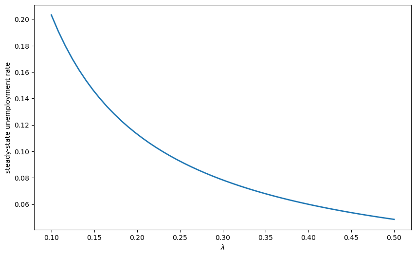
vmapto compute steady states for different parameter valuesPlot how the steady-state unemployment rate varies with the job finding rate \(\lambda\)
Solution to Exercise 69.1
Here is one solution
@jax.jit
def compute_unemployment_rate(λ_val):
    """Computes steady-state unemployment for a given λ"""
    model = LakeModel(λ=λ_val)
    steady_state = rate_steady_state(model)
    return steady_state[0]

# Use vmap to compute for multiple λ values
λ_values = jnp.linspace(0.1, 0.5, 50)
unemployment_rates = jax.vmap(compute_unemployment_rate)(λ_values)

# Plot the results
fig, ax = plt.subplots(figsize=(10, 6))
ax.plot(λ_values, unemployment_rates, lw=2)
ax.set_xlabel(r'$\lambda$')
ax.set_ylabel('steady-state unemployment rate')
plt.show()

model_base = LakeModel()
model_ex1 = LakeModel(α=0.02, λ=0.3)

print(f"Base model α: {model_base.α}")
print(f"New model α: {model_ex1.α}, λ: {model_ex1.λ}")

# Compute steady states for both
base_steady_state = rate_steady_state(model_base)
new_steady_state = rate_steady_state(model_ex1)

print(f"Base unemployment rate: {base_steady_state[0]:.4f}")
print(f"New unemployment rate: {new_steady_state[0]:.4f}")
Base model α: 0.013
New model α: 0.02, λ: 0.3
Base unemployment rate: 0.0827
New unemployment rate: 0.0978
Exercise 69.2
Consider an economy with an initial stock of workers \(N_0 = 100\) at the steady state level of employment in the baseline parameterization
\(\alpha = 0.013\)
\(\lambda = 0.283\)
\(b = 0.0124\)
\(d = 0.00822\)
(The values for \(\alpha\) and \(\lambda\) follow [Davis et al., 2006])
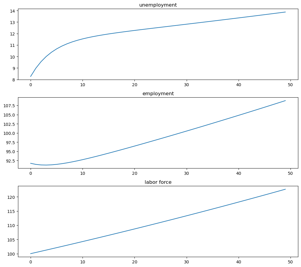
Suppose that in response to new legislation the hiring rate reduces to \(\lambda = 0.2\).
Plot the transition dynamics of the unemployment and employment stocks for 50 periods.
Plot the transition dynamics for the rates.
How long does the economy take to converge to its new steady state?
What is the new steady state level of employment?
Solution to Exercise 69.2
We begin by constructing the model with default parameters and finding the initial steady state
model_initial = LakeModel()
x0 = rate_steady_state(model_initial)
print(f"Initial Steady State: {x0}")
Initial Steady State: [0.08266623 0.9173338 ]
Initialize the simulation values
N0 = 100
T = 50
New legislation changes \(\lambda\) to \(0.2\)
model_ex2 = LakeModel(λ=0.2)
xbar = rate_steady_state(model_ex2)  # new steady state

# Simulate paths
X_path = generate_path(stock_update, x0 * N0, T, model=model_ex2)
x_path = generate_path(rate_update, x0, T, model=model_ex2)
print(f"New Steady State: {xbar}")
New Steady State: [0.1130929 0.8869071]
Now plot stocks
fig, axes = plt.subplots(3, 1, figsize=[10, 9])

axes[0].plot(X_path[0, :])
axes[0].set_title('unemployment')

axes[1].plot(X_path[1, :])
axes[1].set_title('employment')

axes[2].plot(X_path.sum(0))
axes[2].set_title('labor force')

plt.tight_layout()
plt.show()
And how the rates evolve
fig, axes = plt.subplots(2, 1, figsize=(10, 8))

titles = ['unemployment rate', 'employment rate']

for i, title in enumerate(titles):
    axes[i].plot(x_path[i, :])
    axes[i].hlines(xbar[i], 0, T, 'r', '--')
    axes[i].set_title(title)

plt.tight_layout()
plt.show()
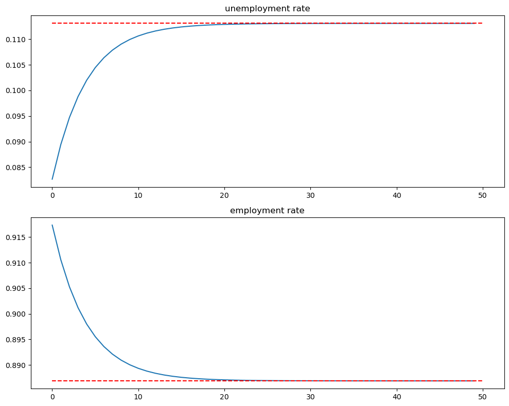
We see that it takes 20 periods for the economy to converge to its new steady state levels.
Exercise 69.3
Consider an economy with an initial stock of workers \(N_0 = 100\) at the steady state level of employment in the baseline parameterization.
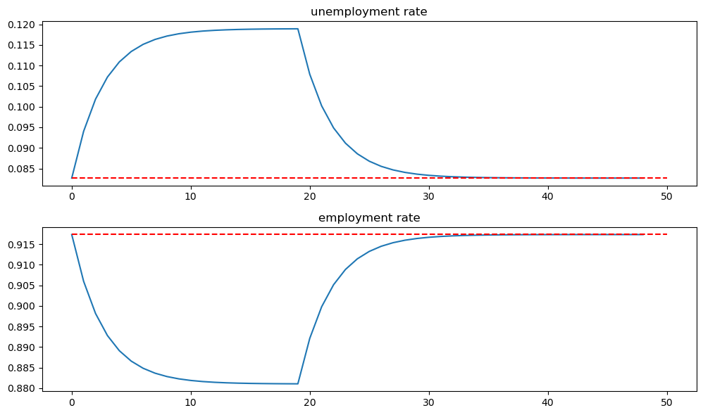
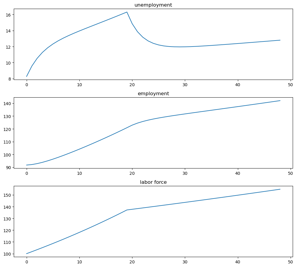
Suppose that for 20 periods the birth rate was temporarily high (\(b = 0.025\)) and then returned to its original level.
Plot the transition dynamics of the unemployment and employment stocks for 50 periods.
Plot the transition dynamics for the rates.
How long does the economy take to return to its original steady state?
Solution to Exercise 69.3
This exercise has the economy experiencing a boom in entrances to the labor market and then later returning to the original levels.
For 20 periods the economy has a new entry rate into the labor market.
Let’s start off at the baseline parameterization and record the steady state
model_baseline = LakeModel()
x0 = rate_steady_state(model_baseline)
N0 = 100
T = 50
Here are the other parameters:
b_hat = 0.025
T_hat = 20
Let’s increase \(b\) to the new value and simulate for 20 periods
model_high_b = LakeModel(b=b_hat)

# Simulate stocks and rates for first 20 periods
X_path1 = generate_path(stock_update, x0 * N0, T_hat, model=model_high_b)
x_path1 = generate_path(rate_update, x0, T_hat, model=model_high_b)
Now we reset \(b\) to the original value and then, using the state after 20 periods for the new initial conditions, we simulate for the additional 30 periods
# Use final state from period 20 as initial condition
X_path2 = generate_path(stock_update, X_path1[:, -1], T-T_hat,
                            model=model_baseline)
x_path2 = generate_path(rate_update, x_path1[:, -1], T-T_hat,
                            model=model_baseline)
Finally, we combine these two paths and plot
# Combine paths
X_path = jnp.hstack([X_path1, X_path2[:, 1:]])
x_path = jnp.hstack([x_path1, x_path2[:, 1:]])

fig, axes = plt.subplots(3, 1, figsize=[10, 9])

axes[0].plot(X_path[0, :])
axes[0].set_title('unemployment')

axes[1].plot(X_path[1, :])
axes[1].set_title('employment')

axes[2].plot(X_path.sum(0))
axes[2].set_title('labor force')

plt.tight_layout()
plt.show()
And the rates
fig, axes = plt.subplots(2, 1, figsize=[10, 6])

titles = ['unemployment rate', 'employment rate']

for i, title in enumerate(titles):
    axes[i].plot(x_path[i, :])
    axes[i].hlines(x0[i], 0, T, 'r', '--')
    axes[i].set_title(title)

plt.tight_layout()
plt.show()